Accumulated Local Effect (ALE)

(Feature Influence)

Kacper Sokol

Topics

• Method Overview
• (Algorithmic) Building Blocks
• Theoretical Underpinning
• Variants
• Examples
• Case Studies & Gotchas!
• Properties
• Further Considerations

Method Overview

Explanation Synopsis

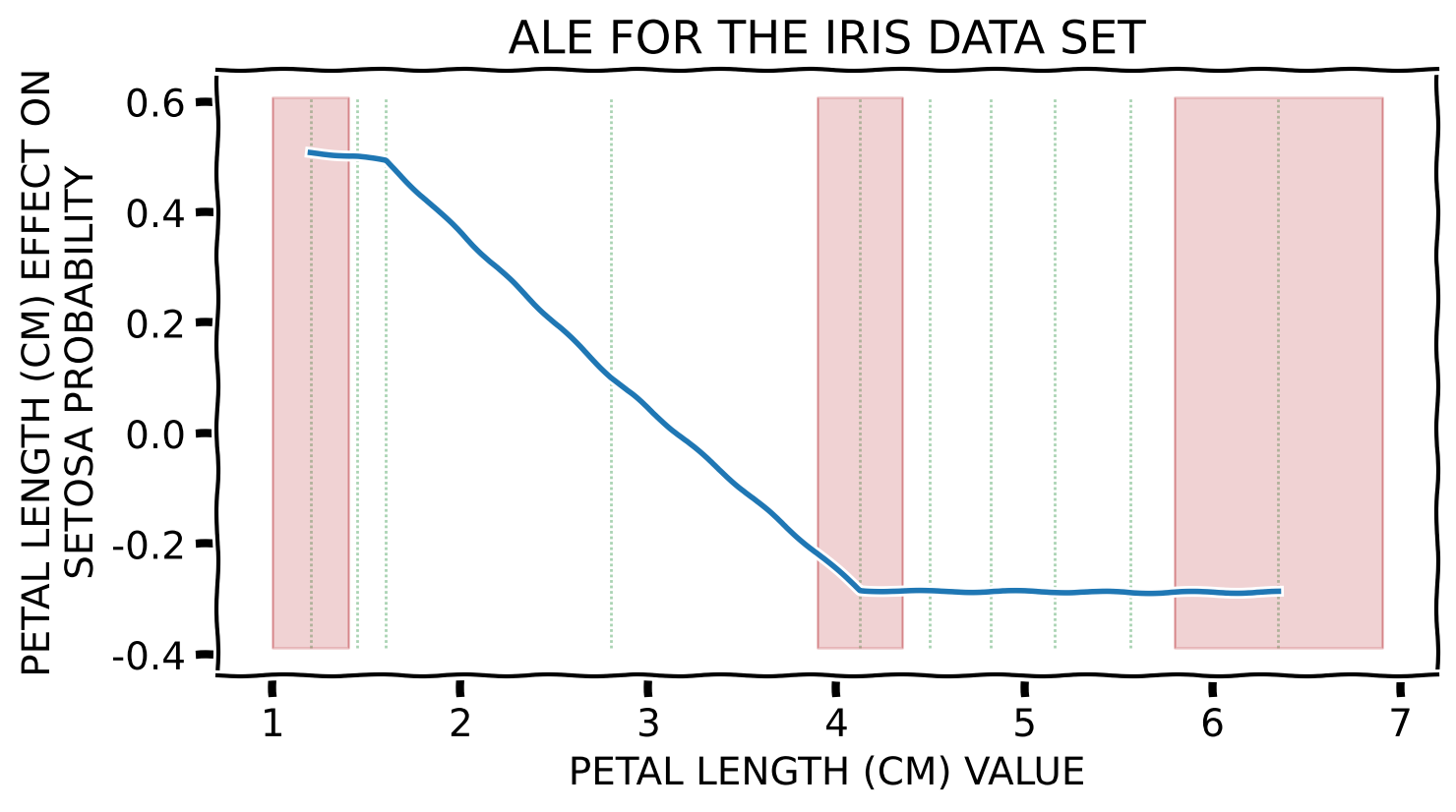
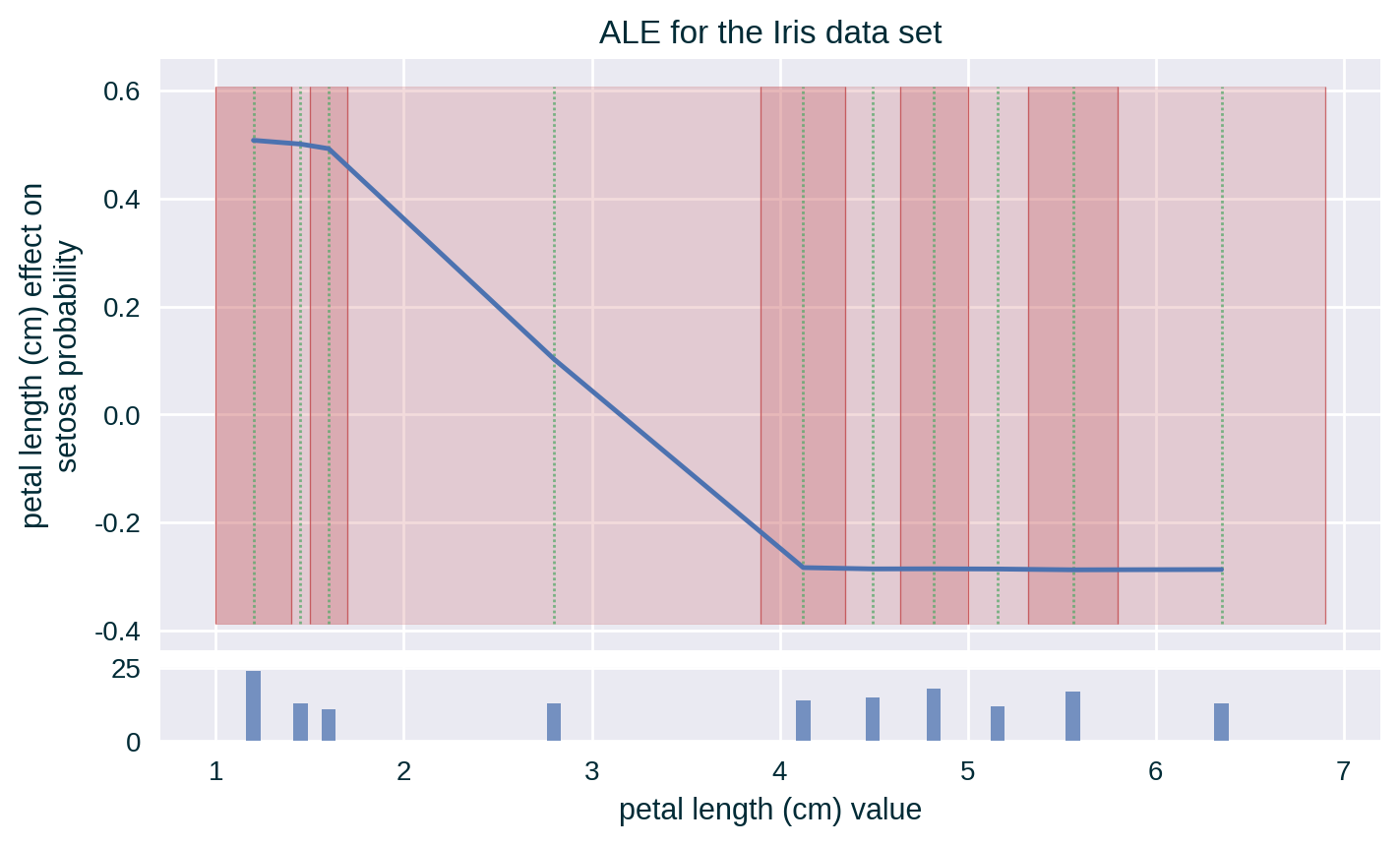
ALE captures the influence of a specific feature value on the model’s prediction by quantifying the average (accumulated) difference between the predictions at the boundaries of a (small) fixed interval around the selected feature value (Apley and Zhu 2020). It is calculated by replacing the value of the explained feature with the interval boundaries for instances found in the designated data set whose value of this feature is within the specified range.

It communicates global (with respect to the entire explained model) feature influence.

Rationale

ALE is an evolved version of (relaxed) Marginal Effect (ME) (Apley and Zhu 2020) that is less prone to being affected by feature correlation since it relies upon average prediction change. It also improves upon Partial Dependence (PD) (Friedman 2001) by ensuring that the influence estimates are based on realistic instances (thus respecting interactions between features / feature correlation), making the explanatory insights more truthful.

Toy Example – Numerical Feature

• ALE values is the change in the output of the predictive model – probability of a particular class here – within feature partitions over the range of the feature, in reference to the average prediction

• ALE values can be interpreted as the (main) effect of the feature at a certain value (middle of the bin) compared to its average effect; e.g., the estimate of +0.15 at petal length (cm) 2.75, communicates that for this particular feature value the effect is higher by 0.15 than the average effect of -0.59

Method Properties

Property	Accumulated Local Effect
relation	post-hoc
compatibility	model-agnostic
modelling	regression and probabilistic classification (numbers)
scope	global (per data set; generalises to cohort)
target	model (set of predictions)

• Because of the difference in prediction at bin boundaries, ALE does not work with crisp classifiers

Method Properties    

Property	Accumulated Local Effect
data	tabular
features	numerical (ordinal categorical)
explanation	feature influence (visualisation)
caveats	feature binning

• Because of pushing instances to bin boundaries created for the explained feature – to calculate the difference in prediction at these two points – ALE does not work with categorical features out of the box
• This limitation can be overcome by establishing an order among categorical features
• For example, the order can be induced by comparing similarity between categories based on other feature values

(Algorithmic) Building Blocks

Computing ALE

Input

1. Select a feature to explain

2. Select the explanation target

   • probabilistic classifiers → (probabilities of) one class
   • regressors → numerical values

3. Select a collection of instances to generate the explanation

Computing ALE    

Parameters

1. Define binning of the explained (numerical) feature

   • select the number of bins
   • decide on fixed-width, quantile or custom binning

Computing ALE    

Procedure

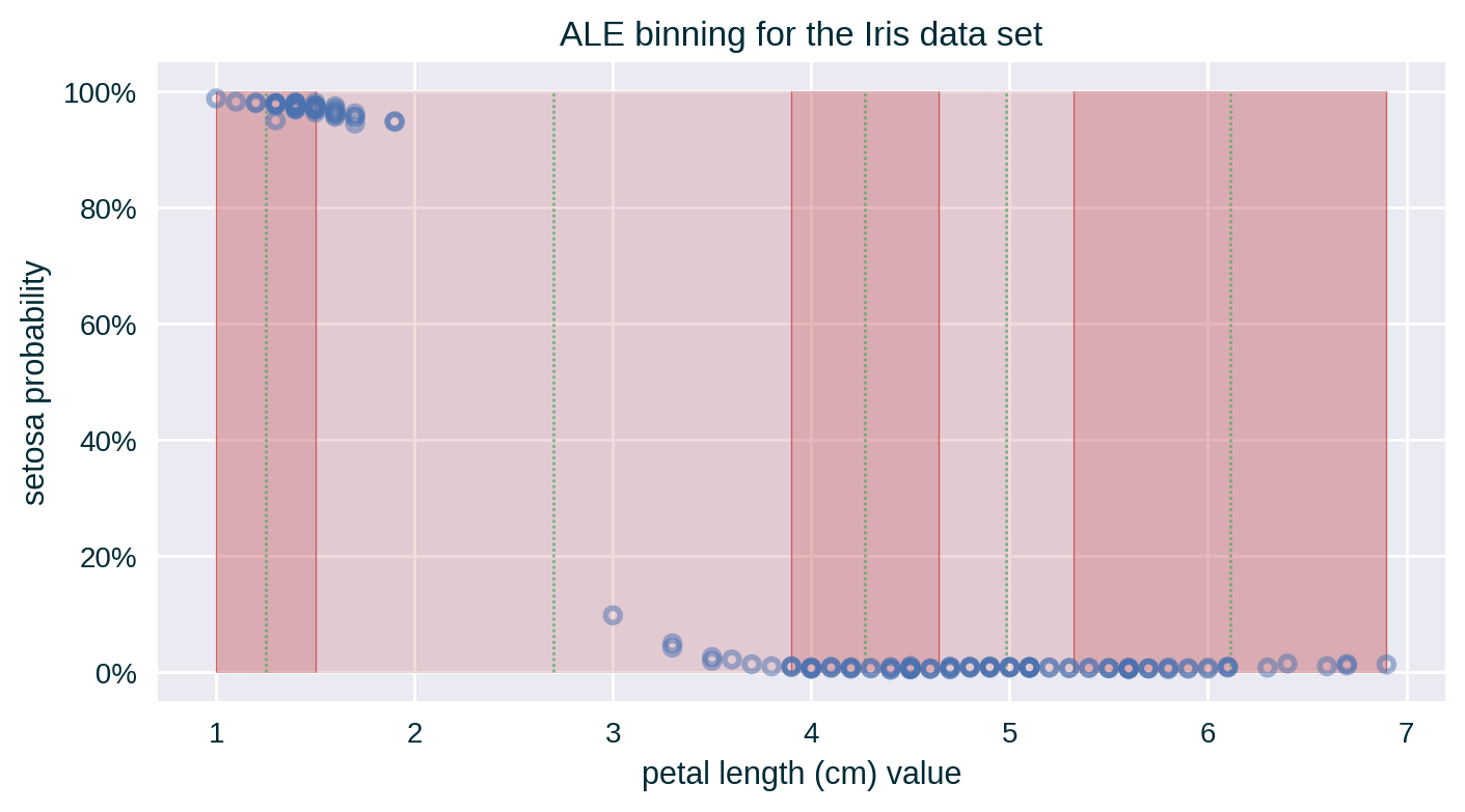
1. For each instance in the designated data set, assign it to a bin that spans the range to which the value of its explained feature belongs

Computing ALE    

Computing ALE    

Procedure    

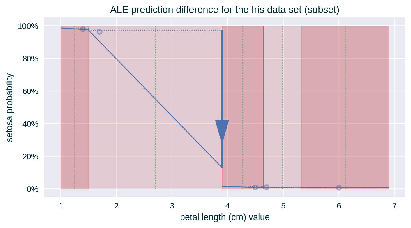
2. For each instance in each bin, calculate the difference between the prediction of these instances at bin boundaries

Computing ALE    

Computing ALE    

Procedure    

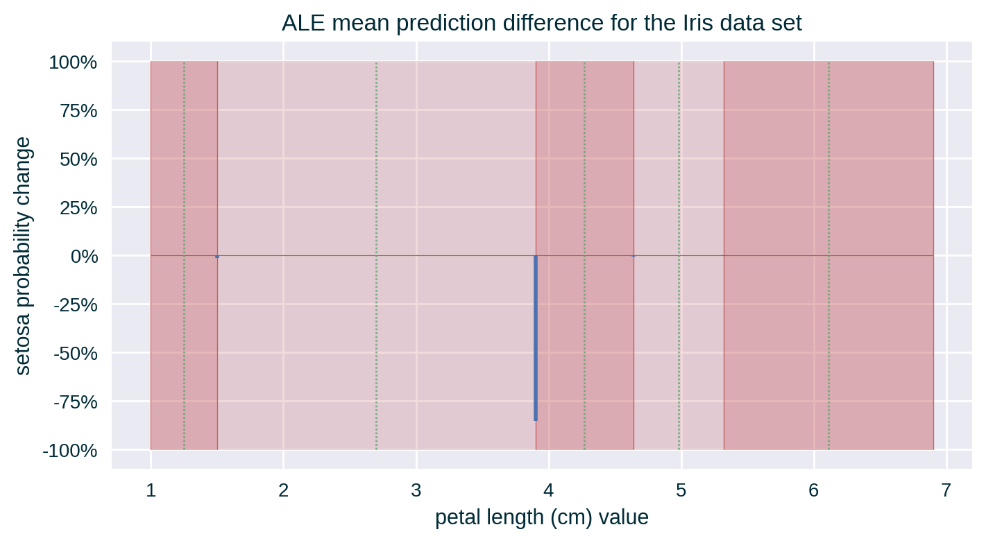
3. Calculate the mean change in prediction for each bin

Computing ALE    

Computing ALE    

Procedure    

4. Accumulate the mean change in prediction over the bins

Computing ALE    

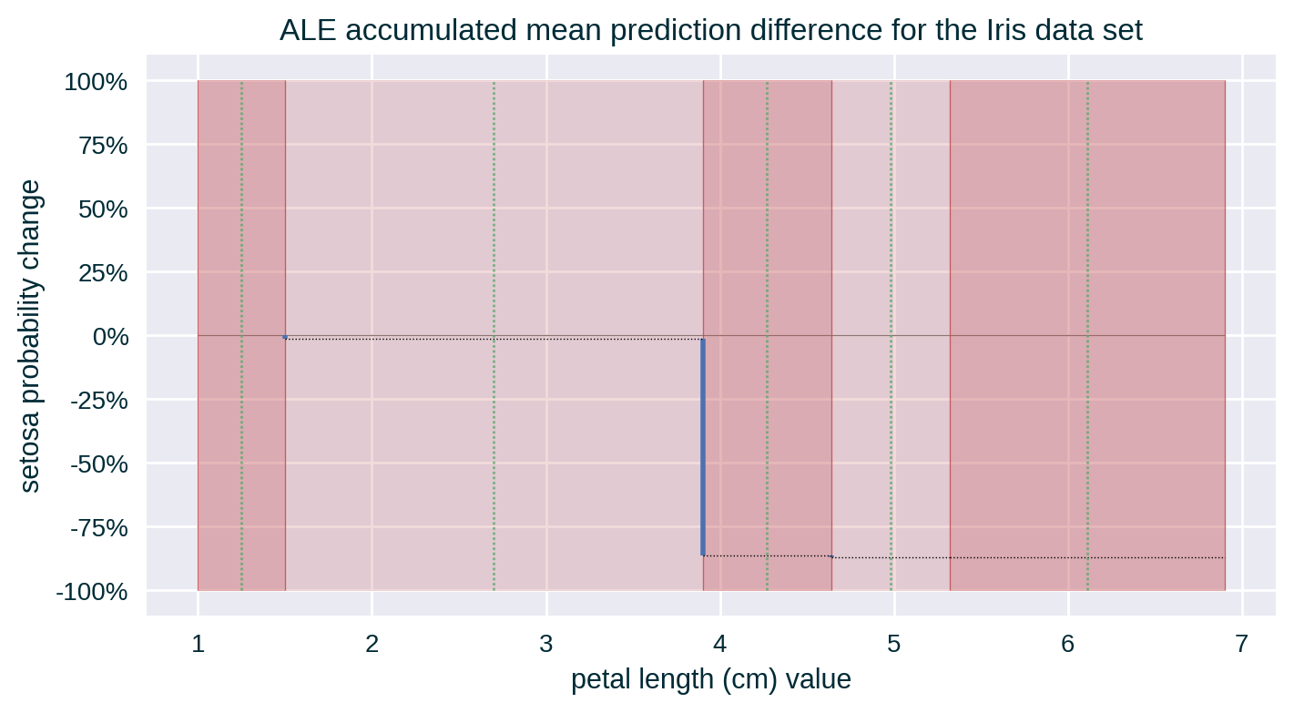
Computing ALE    

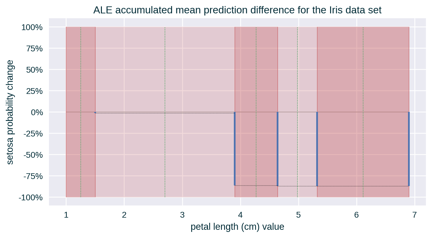
Computing ALE    

Procedure    

5. Extrapolate the value of the accumulated mean change in prediction in the middle of each bin

Computing ALE    

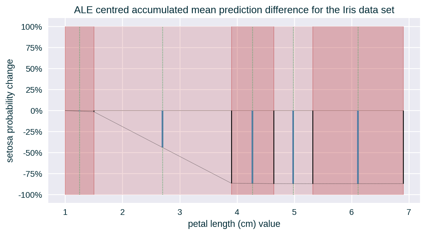
Computing ALE    

Procedure    

6. Centre (the extrapolated value of) the accumulated mean change in prediction in the middle of each bin around their mean

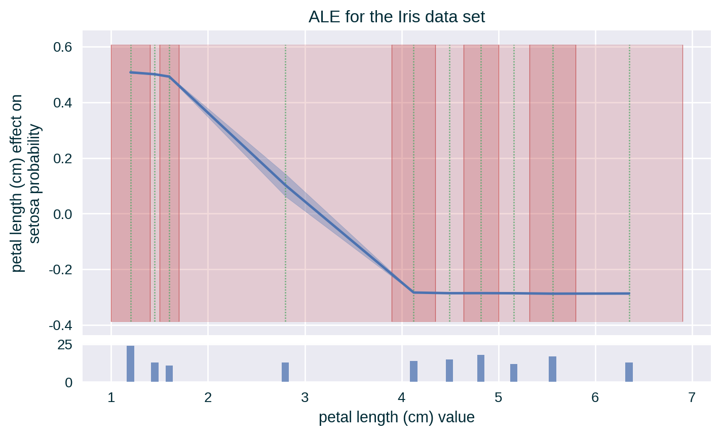
    Depending on the binning strategy, the number of instances per bin may be distributed unevenly. A histogram representing the number of instances in each bin can help in interpreting the explanation.

• Quantile binning offers even distribution of instances per bin, but may result in bins of disparate lengths
• Other binning may result in underrepresented bins

Computing ALE    

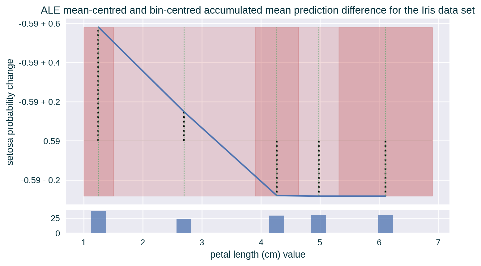
Theoretical Underpinning

Formulation    

\[ X_{\mathit{ALE}} \subseteq \mathcal{X} \]

\[ V_i = \{ x_i : x \in X_{\mathit{ALE}} \} \]

\[ \mathit{ALE}_i = \int_{v_{0}}^{x_i} \mathbb{E}_{X_{\setminus i} | X_{i}=x_i} \left[ f^i \left( X_{\setminus i} , X_{i} \right) | X_{i}=v_i \right] \; d v_i - \mathit{const} \\ \;\;\;\;\;\;\;\;\;\;\;\;\;\;\;\;= \int_{v_{0}}^{x_i} \left ( \int_{X_{\setminus i}} f^i \left( X_{\setminus i} , v_i \right) \; d \mathbb{P} ( X_{\setminus i} | X_i = v_i ) \right ) \; d v_i - \mathit{const} \]

\[ f^i (x_{\setminus i}, x_i) = \frac{\partial f (x_{\setminus i}, x_i)}{\partial x_i} \]

• There are 2 differences between this formulation and ME formulation

  • \(f\) is replaced with \(f^i\) to reflect that we are interested in the (average [expected]) change of prediction when \(x_i\) changes
  • the outer integral \(\int_{v_{0}}^{x_i}\) captures the accumulation over values \(v_0, \ldots x_i\) – from minimum up to the value for that feature of the explained instace – for the feature \(x_i\) (in computation these become discrete intervals)

• The outer integral and the partial derivative in conjunction ensure that we isolate the effect of the explained feature from other features

• By subtracting a constant (\(\mathit{const}\)) we centre ALE such that the average effect is 0

• Conditioning the difference in predictions on the distribution of the explained feature(s) yields (average) effect of the explained feature(s) (and this feature alone) on predictions

Formulation        

Based on the ICE notation (Goldstein et al. 2015)

\[ \hat{f}_S = \int_{z_{0, S}}^{x_S} \mathbb{E}_{X_{C} | X_S = x_S} \left[ \hat{f}^{S} \left( X_{S} , X_{C} \right) | X_S = z_S \right] \; d z_{S} - \mathit{const} \\ \;\;\;\;\;\;\;\;= \int_{z_{0, S}}^{x_S} \left ( \int_{X_C} \hat{f}^{S} \left( z_{S} , X_{C} \right) \; d \mathbb{P} ( X_{C} | X_S = z_S ) \right ) \; d z_{S} - \mathit{const} \]

\[ \hat{f}^{S} (x_s, x_c) = \frac{\partial \hat{f} (x_S, x_C)}{\partial x_S} \]

• There are 2 differences between this formulation and ME formulation

  • \(\hat{f}\) is replaced with \(\hat{f}^{S}\) to reflect that we are interested in the (average [expected]) change of prediction when \(x_S\) changes
  • the outer integral \(\int_{z_{0, S}}^{x_S}\) captures the accumulation over values \(z_0, \ldots x_S\) – from minimum up to the value for that feature of the explained instace – for the feature \(X_S\) (in computation these become discrete intervals)

• The outer integral and the partial derivative in conjunction ensure that we isolate the effect of the explained feature from other features

• By subtracting a constant (\(\mathit{const}\)) we centre ALE such that the average effect is 0

• \(x_S\) is fixed – the explained feature

• \(x_C\) are the given feature values

• \(X_C\) and \(X_S\) are the random variables

• Conditioning the difference in predictions on the distribution of the explained feature(s) yields (average) effect of the explained feature(s) (and this feature alone) on predictions

Approximation    

\[ \mathit{ALE}_i^{j} \approx \sum_{n=1}^{j} \frac{1}{|Z_n|} \sum_{x \in Z_n} \left[ f \left( x_{\setminus i} , x_i=Z_n^+ \right) - f \left( x_{\setminus i} , x_i=Z_n^- \right) \right] \]

\[ \overline{\mathit{ALE}_i^{j}} = \mathit{ALE}_i^{j} - \frac{1}{\sum_{Z_n \in Z} |Z_n|} \sum_{x \in Z} \mathit{ALE}_i(x) \]

• The top one is uncentred; the bottom one is centred (no \(j\) superscript in \(\mathit{ALE}_i\) means that we go to the interval where the instance \(x\) is located)

• \(\mathit{ALE}_i^j\) – ALE of feature \(i\) for interval \(j\)

• \(Z_n\) is the \(n\)-th interval; \(Z_n^-\) is the lower bound of the \(n\)-th interval; and \(Z_n^+\) is the upper bound of the \(n\)-th interval

• Since we may not have access to gradient ([partial] derivative) of the predictive function, we use difference over intervals (approximation)

• effect is the difference in prediction in a given interval, which makes it local; we accumulate this effect up to inteval \(j\)

Variants

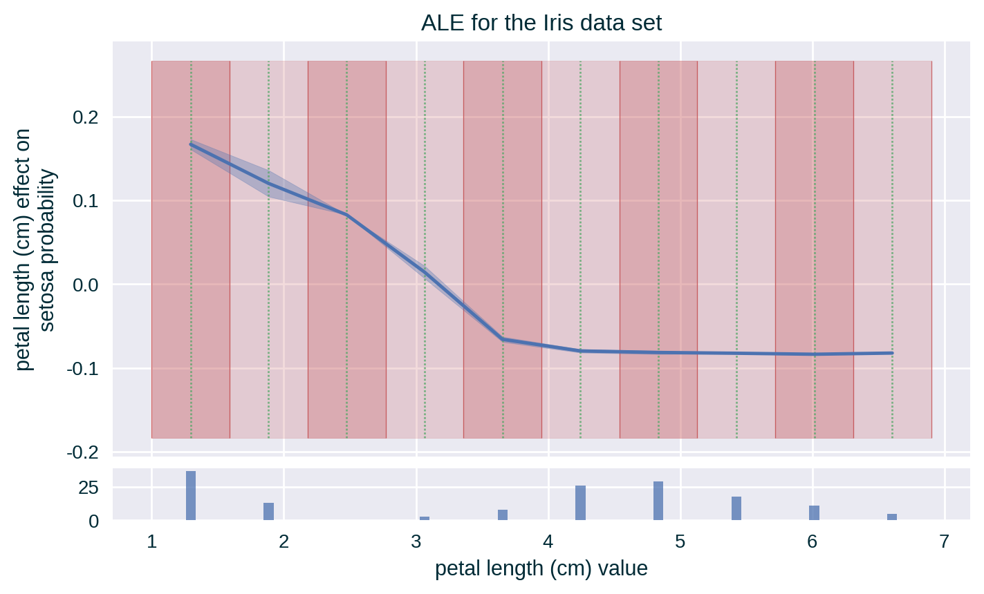
Feature Binning Approaches

Given the need for binning, various approaches such as:

• quantile,
• equal-width or
• custom.

can be used.

(Examples to follow.)

Multi-dimensional ALE

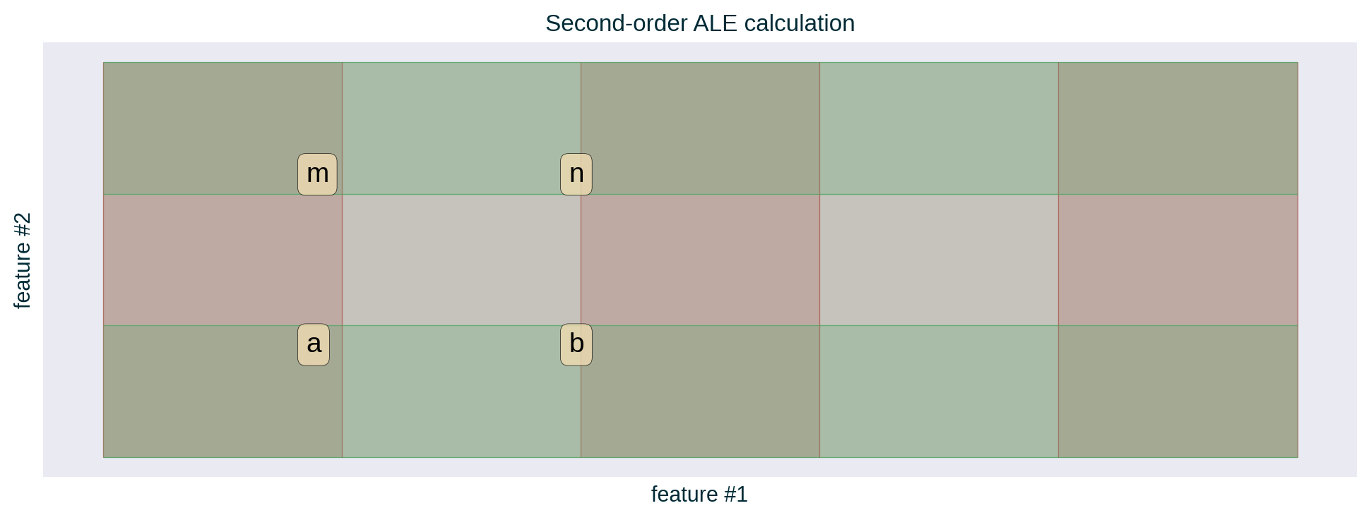
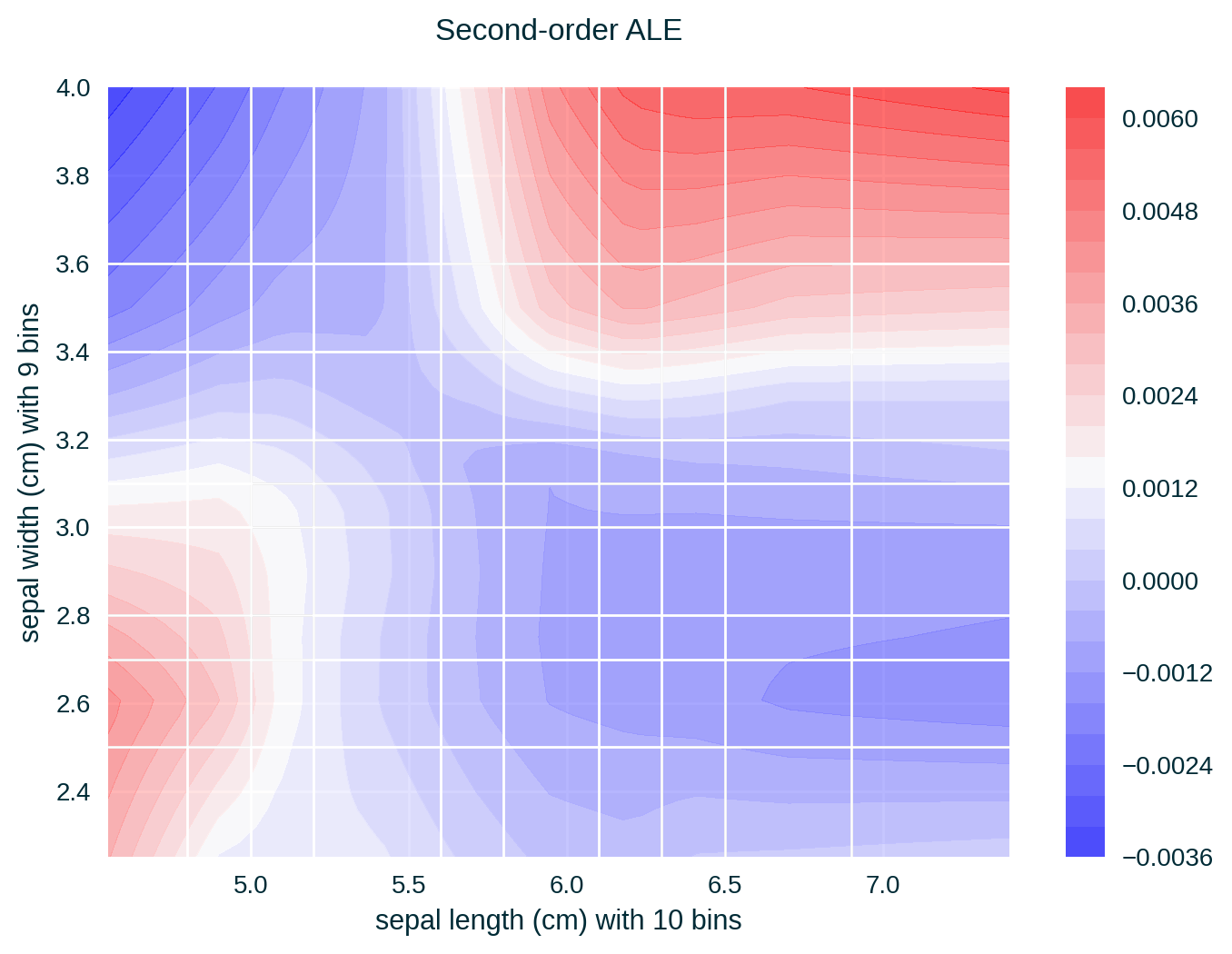
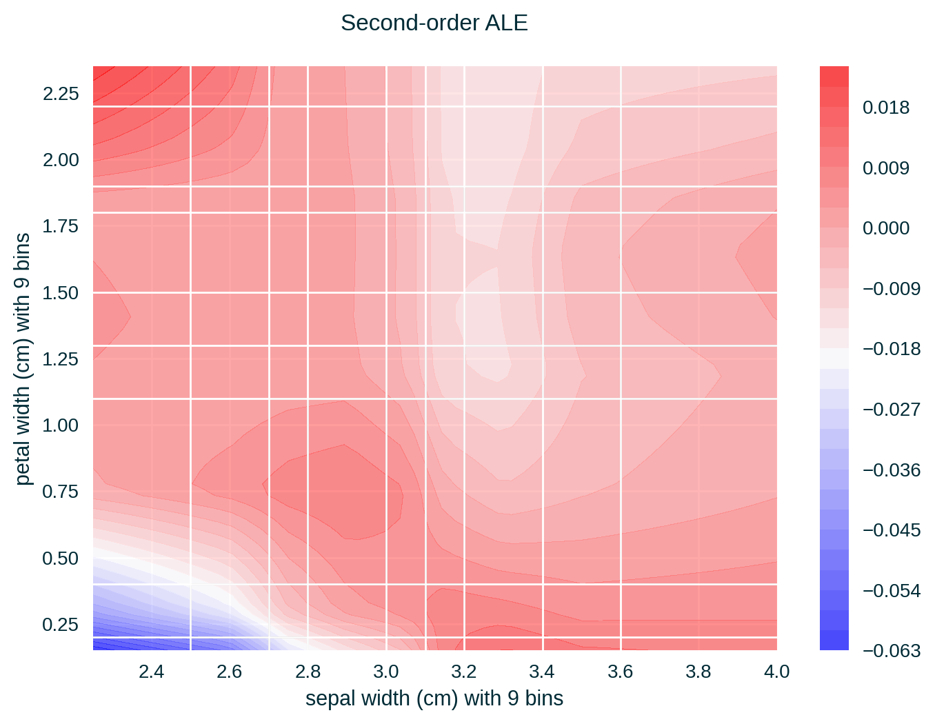
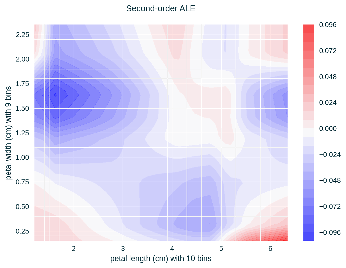
ALE of a single feature captures only the effect of this particular feature on the explained model’s predictive behaviour – known as first-order effect. ALE of multiple features capture the exclusive effect of the interaction between n features on the explained model’s predictive behaviour (adjusted for the overall effect as well as the main effect of each feature) – known as n^th-order effect, e.g., second-order effect.

(Examples to follow.)

Formulation    

Refer to Apley and Zhu (2020) for the formulation.

Multi-dimensional ALE    

Computation    

\[ \underbrace{ \overbrace{(n - m)}^{\text{feature #1}} - \overbrace{(b - a)}^{\text{feature #1}} }_{\text{feature #2}} \]

Examples

ALE

ALE with Standard Deviation

Uniform Binning ALE (with Standard Deviation)

ALE for Two Features

Case Studies & Gotchas!

Feature Correlation

• If a feature has not effect on the prediction (in a given section of a feature), it shows in ALE as a straight line
• ALE is centred around 0 if it has no effect on the feature throughout the entire range
• Since the underlying model is linear, features are assumed to be independent and have linear effect on the prediction

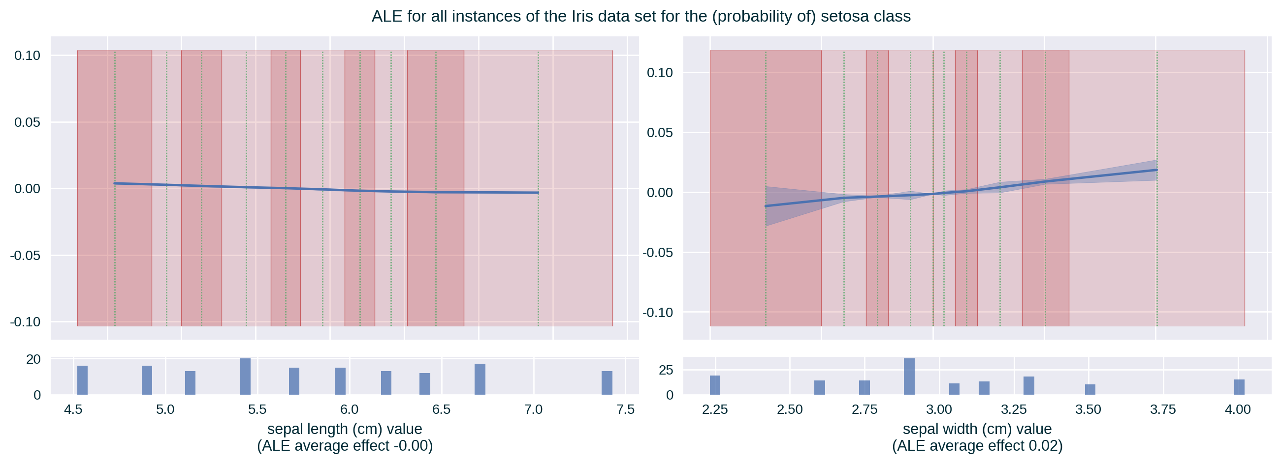
Feature Correlation    

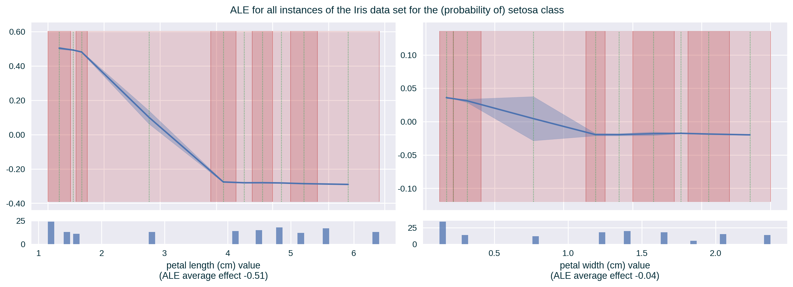
Feature Correlation    

• This agrees with the insights communicated by ALE – despite diverse predictions, indiviudal response is quite stable

• Note: By design, PD reports the total (all, up to the n^th-order effects), but ALE separates effects of a given order

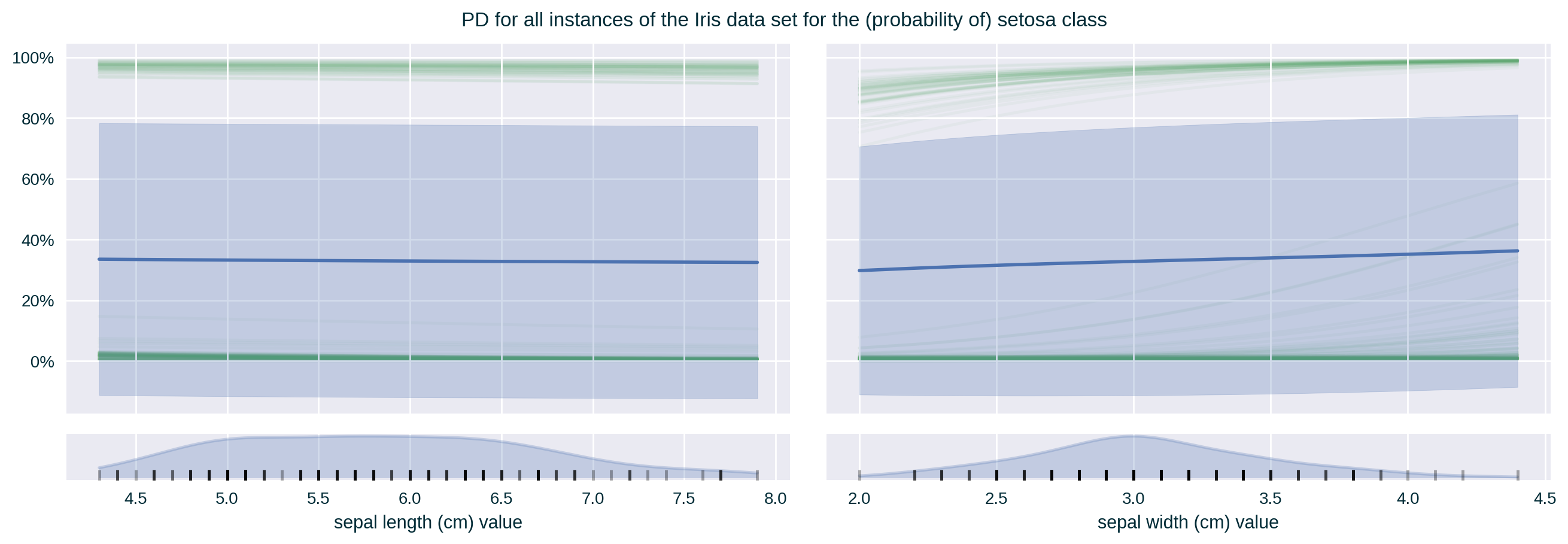
Feature Correlation    

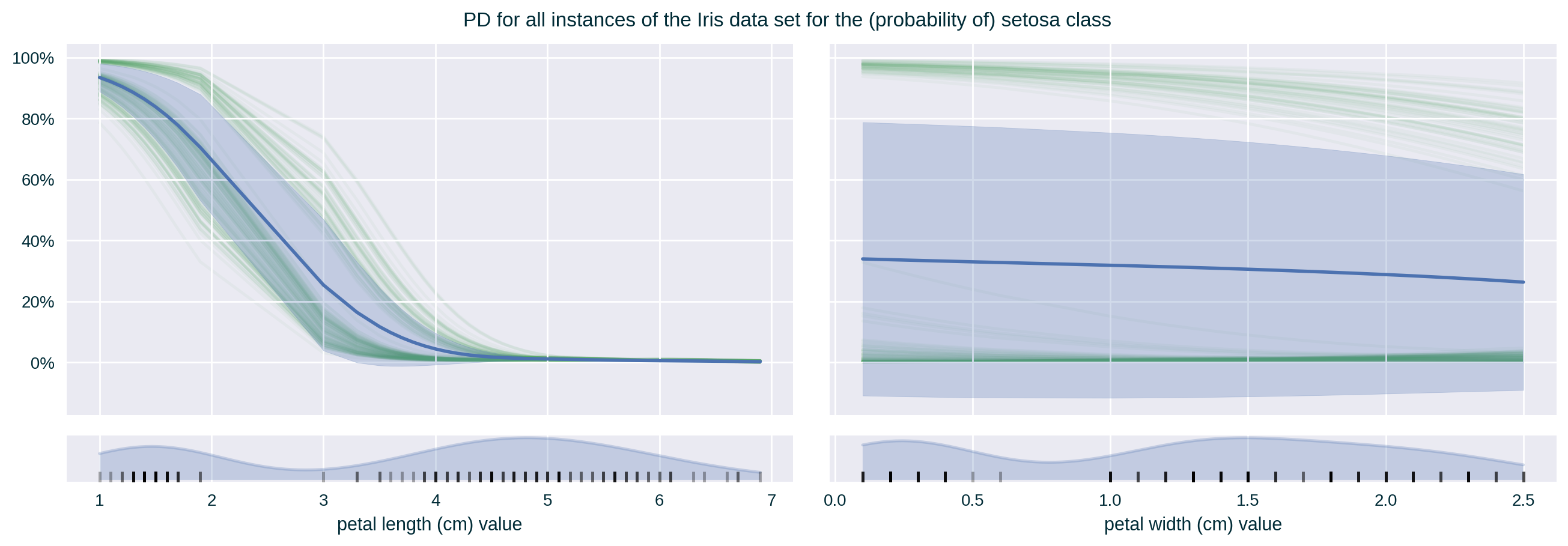
Feature Correlation    

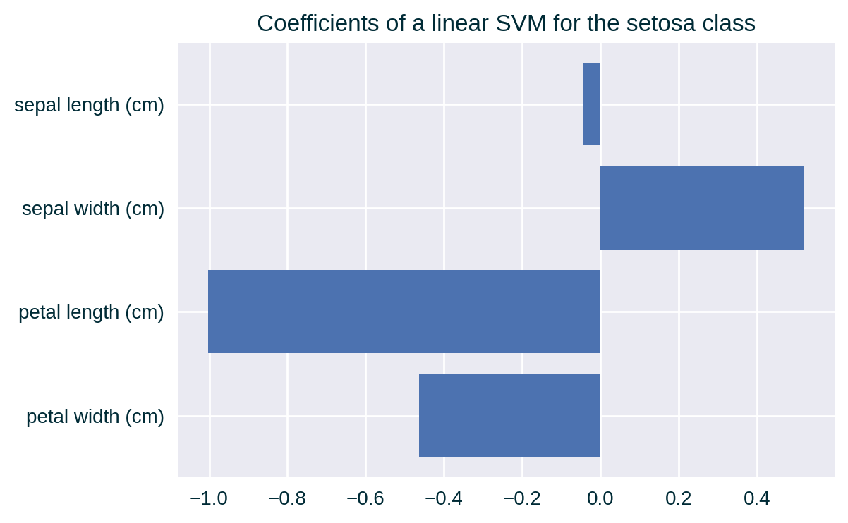
ALE and Linear Model Coefficients

See Grömping (2020) for an explanation why ALE may not reflect the coefficients of a linear model.

• But based on the model coefficients, we can see that other features contribute to the prediction

Feature Correlation    

• These somewhat counterintuitive explanations are caused by strong feature correlation

Feature Correlation    

• Recall: Second-order effect communicates the additional effect due to interaction between two features on the predictions of the explained model, after accoutning for the main effect of both features
• Most of second-order effects are close to 0

Feature Correlation    

Feature Correlation    

Feature Correlation    

• The negative effect of this second-order ALE is non-negligible (albeit in a small region of the feature grid)

• While the undelrying model is linear and presupposes no feature interaction, the feature correlation cannot be ignored

• While petal length (cm) is the main predictive feature, its interaction with sepal width (cm) in a small region helps to predict the classes

• petal length (cm) – y-axis – is influential in first-order ALE and strongly correlated (mostly positive) with

  • sepal length (cm) (+0.87)
  • petal width (cm) (+0.96)
  • sepal width (cm) (-0.43)

• sepal width (cm) – x-axis – is weakly correlated (negative) with

  • sepal length (cm) (-0.12)
  • petal width (cm) (-0.43)
  • sepal length (cm) (-0.37)

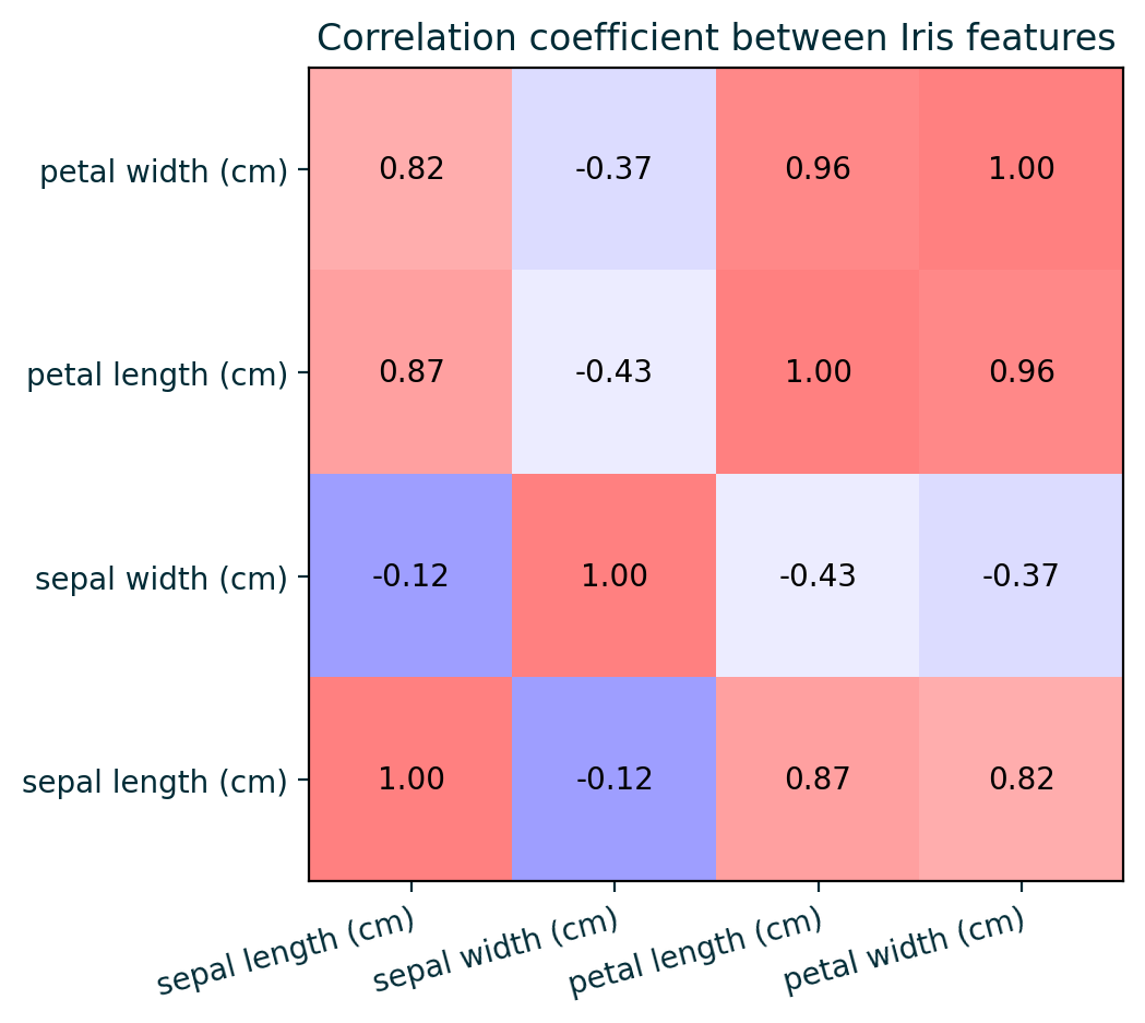
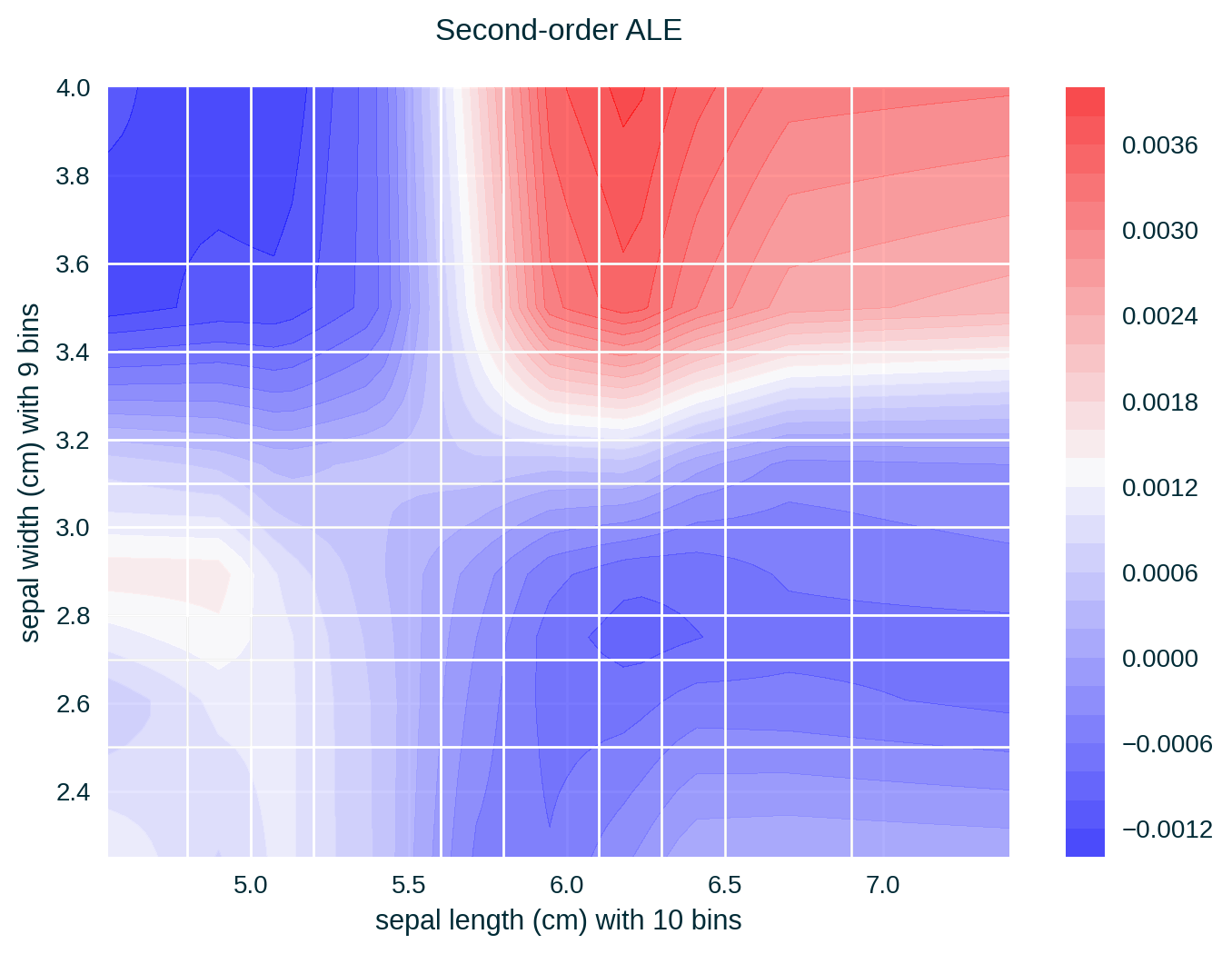
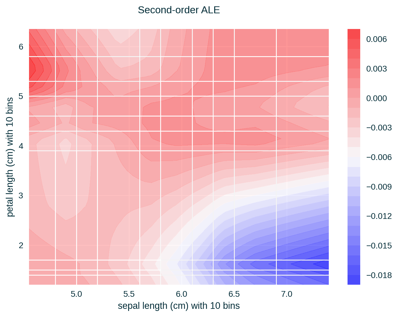
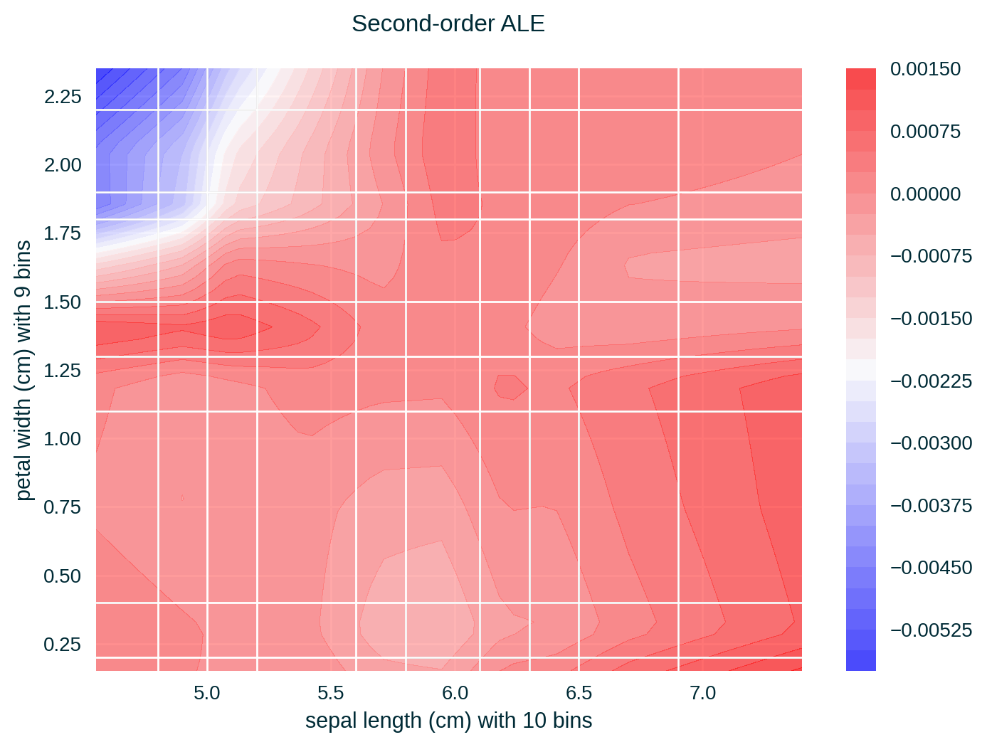
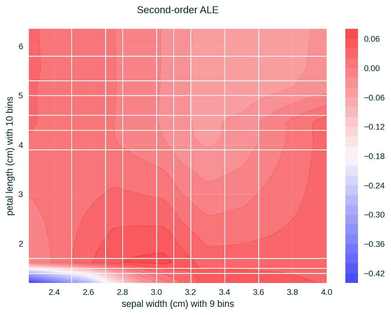
Feature Correlation    

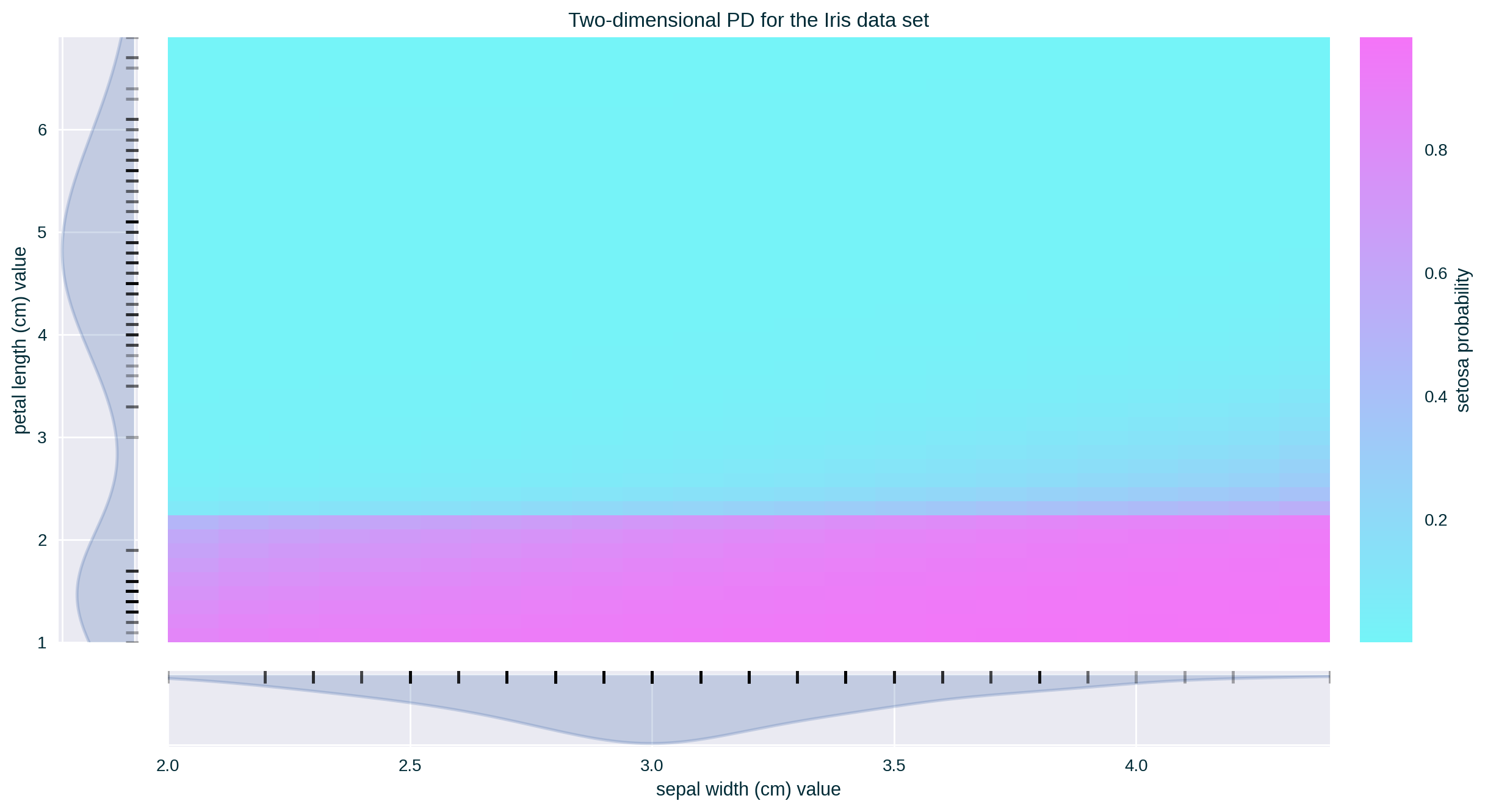
Feature Correlation    

Feature Correlation    

Properties

Pros    

• Easy and fast to generate

• Reasonably easy to interpret (first-order ALE)

• Reliable when features are correlated (unbiased)

• Based on data that are closely distributed to the real data

Cons    

• Not so easy to implement

• Tricky to interpret for orders higher than first

• Limited to explaining two feature at a time

• ALE trends should not be generalised to individual instances across the feature range since the estimates are specific to each bin

Cons        

• Binning may skew the results (aided by displaying distribution of instances per bin); e.g.,

  • quantiles ensure good estimates given the number of instances per bin, but may yield unusually long and short bins;
  • fixed-width offers regular bins, but some may lack a sufficient number of points to offer reliable estimates

Caveats    

• The measurements may be sensitive to different binning approaches
• Computational complexity: \(\mathcal{O} \left( n \right)\), where \(n\) is the number of instances in the designated data set

Further Considerations

Related Techniques

Marginal Effect (ME)

    ME captures the average response of a predictive model across a collection of instances (taken from a designated data set) for a specific value of a selected feature (found in the aforementioned data set) (Apley and Zhu 2020). When relaxed by including similar feature values determined by a fixed interval around the selected value, this method offers similar insights to ALE: average prediction per interval instead of (accumulated) difference in prediction per interval.

Related Techniques    

Individual Conditional Expectation (ICE)

    It communicates the influence of a specific feature value on the model’s prediction by fixing the value of this feature across a designated range for a selected data point (Goldstein et al. 2015). It is an instance-focused (local) “variant” of Partial Dependence.

Related Techniques    

Partial Dependence (PD)

    It communicates the average influence of a specific feature value on the model’s prediction by fixing the value of this feature across a designated range for a set of instances. It is a model-focused (global) “variant” of Individual Conditional Expectation, which is calculated by averaging ICE across a collection of data points (Friedman 2001).

Implementations

Python	R
ALEPython	ALEPlot
alibi	DALEX
	iml

Further Reading

• ALE paper (Apley and Zhu 2020)
• Interpretable Machine Learning book
• Explanatory Model Analysis book

Bibliography

Apley, Daniel W, and Jingyu Zhu. 2020. “Visualizing the Effects of Predictor Variables in Black Box Supervised Learning Models.” Journal of the Royal Statistical Society: Series B (Statistical Methodology) 82 (4): 1059–86.

Friedman, Jerome H. 2001. “Greedy Function Approximation: A Gradient Boosting Machine.” Annals of Statistics, 1189–1232.

Goldstein, Alex, Adam Kapelner, Justin Bleich, and Emil Pitkin. 2015. “Peeking Inside the Black Box: Visualizing Statistical Learning with Plots of Individual Conditional Expectation.” Journal of Computational and Graphical Statistics 24 (1): 44–65.

Grömping, Ulrike. 2020. “Model-Agnostic Effects Plots for Interpreting Machine Learning Models.” Reports in Mathematics, Physics and Chemistry, Department II, Beuth University of Applied Sciences Berlin Report 1.