
Partial Dependence (PD)
(Feature Influence)
Method Overview
Explanation Synopsis
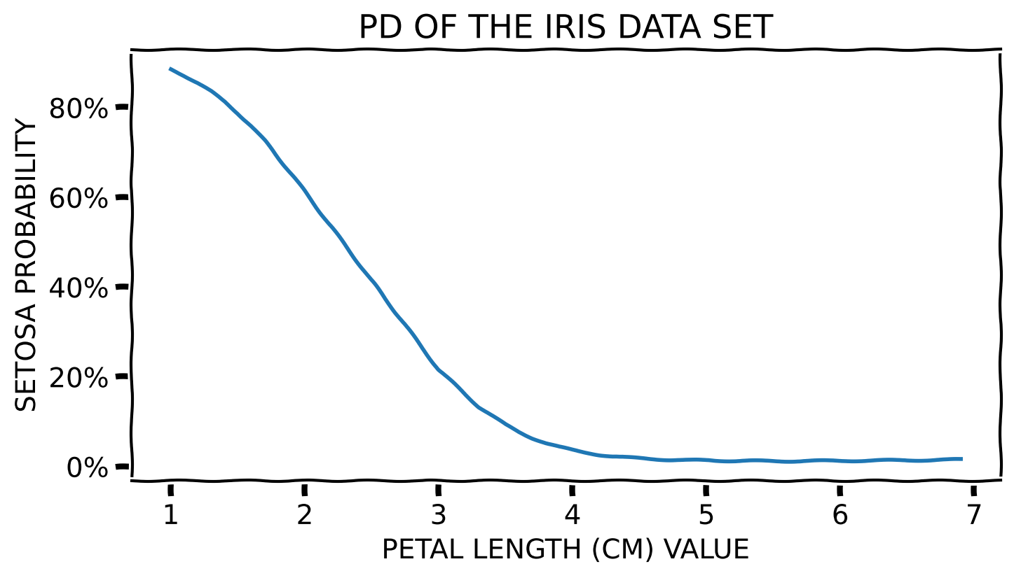
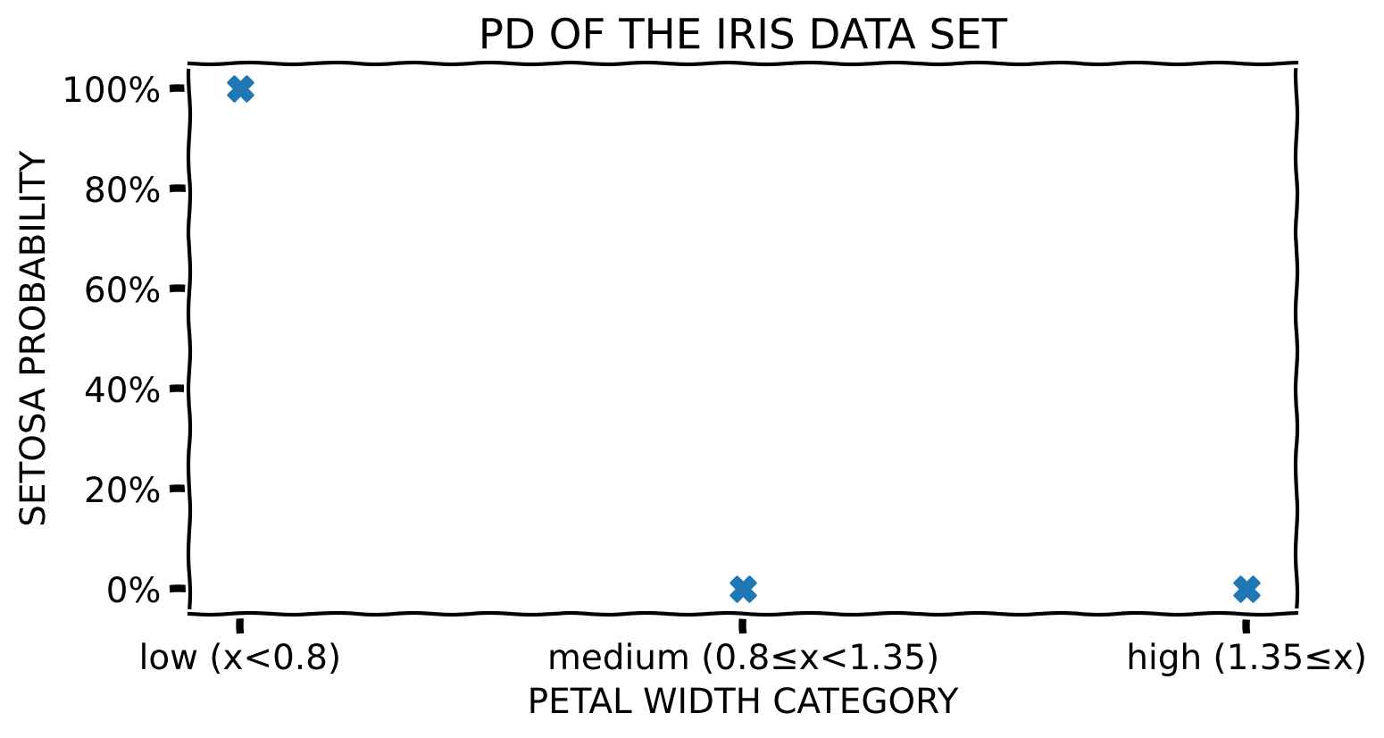
PD captures the average response of a predictive model for a collection of instances when varying one of their features (Friedman 2001).
It communicates global (with respect to the entire explained model) feature influence.
Toy Example – Numerical Feature
Toy Example – Categorical Feature
Method Properties
| Property | Partial Dependence |
|---|---|
| relation | post-hoc |
| compatibility | model-agnostic |
| modelling | regression, crisp and probabilistic classification |
| scope | global (per data set; generalises to cohort) |
| target | model (set of predictions) |
Method Properties
| Property | Partial Dependence |
|---|---|
| data | tabular |
| features | numerical and categorical |
| explanation | feature influence (visualisation) |
| caveats | feature correlation, unrealistic instances, heterogeneous model response |
(Algorithmic) Building Blocks
Computing PD
Input
Select a feature to explain
Select the explanation target
- crisp classifiers → one(-vs.-the-rest) or all classes
- probabilistic classifiers → (probabilities of) one class
- regressors → numerical values
Select a collection of instances to generate the explanation
Computing PD
Parameters
Define granularity of the explained feature
- numerical attributes → select the range – minimum and maximum value – and the step size of the feature
- categorical attributes → the full set or a subset of possible values
Computing PD
Procedure
For each instance in the designated data set create its copy with the value of the explained feature replaced by the range of values determined by the explanation granularity
Predict the augmented data
Generate and plot Partial Dependence
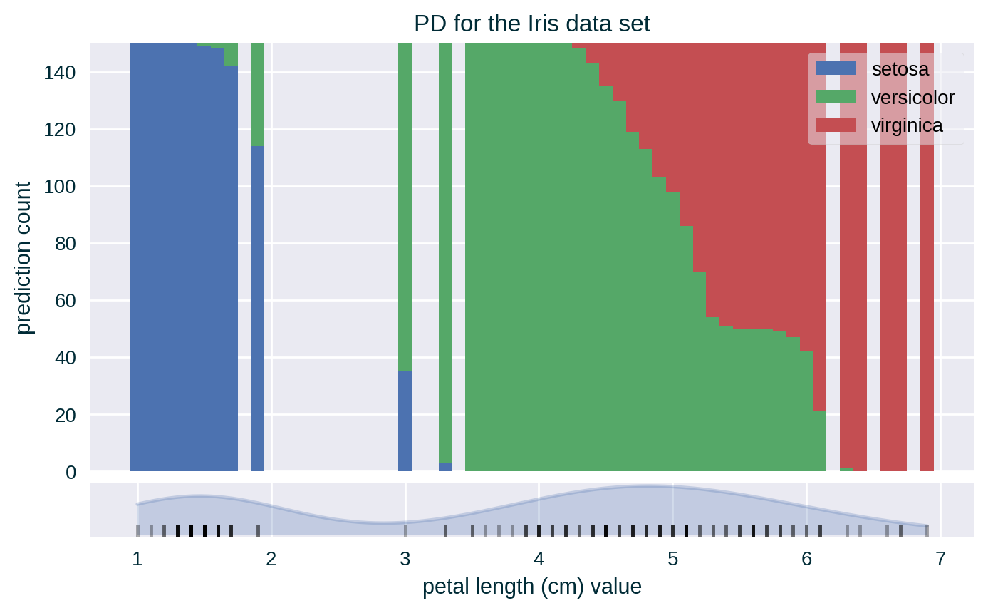
- for crisp classifiers count the number of each unique prediction at each value of the explained feature across all the instances; visualise PD either as a count or proportion using separate line for each class or using a stacked bar chart
- for probabilistic classifiers (per class) and regressors average the response of the model at each value of the explained feature across all the instances; visualise PD as a line
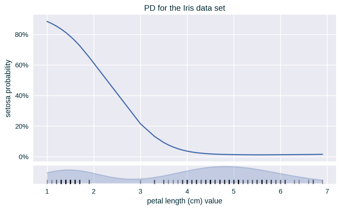
Since the values of the explained feature may not be uniformly distributed in the underlying data set, a rug plot showing the distribution of its feature values can help in interpreting the explanation.
Theoretical Underpinning
Formulation
\[ X_{\mathit{PD}} \subseteq \mathcal{X} \]
\[ V_i = \{ v_i^{\mathit{min}} , \ldots , v_i^{\mathit{max}} \} \]
\[ \mathit{PD}_i = \mathbb{E}_{X_{\setminus i}} \left[ f \left( X_{\setminus i} , x_i=v_i \right) \right] = \int f \left( X_{\setminus i} , x_i=v_i \right) \; d \mathbb{P} ( X_{\setminus i} ) \;\; \forall \; v_i \in V_i \]
\[ \mathit{PD}_i = \mathbb{E}_{X_{\setminus i}} \left[ f \left( X_{\setminus i} , x_i=V_i \right) \right] = \int f \left( X_{\setminus i} , x_i=V_i \right) \; d \mathbb{P} ( X_{\setminus i} ) \]
Formulation
Based on the ICE notation (Goldstein et al. 2015)
\[ \left\{ \left( x_{S}^{(i)} , x_{C}^{(i)} \right) \right\}_{i=1}^N \]
\[ \hat{f}_S = \mathbb{E}_{X_{C}} \left[ \hat{f} \left( x_{S} , X_{C} \right) \right] = \int \hat{f} \left( x_{S} , X_{C} \right) \; d \mathbb{P} ( X_{C} ) \]
Approximation
(Monte Carlo approximation)
\[ \mathit{PD}_i \approx \frac{1}{|X_{\mathit{PD}}|} \sum_{x \in X_{\mathit{PD}}} f \left( x_ {\setminus i} , x_i=v_i \right) \]
\[ \hat{f}_S \approx \frac{1}{N} \sum_{i = 1}^N \hat{f} \left( x_{S} , x_{C}^{(i)} \right) \]
Variants
Centred PD
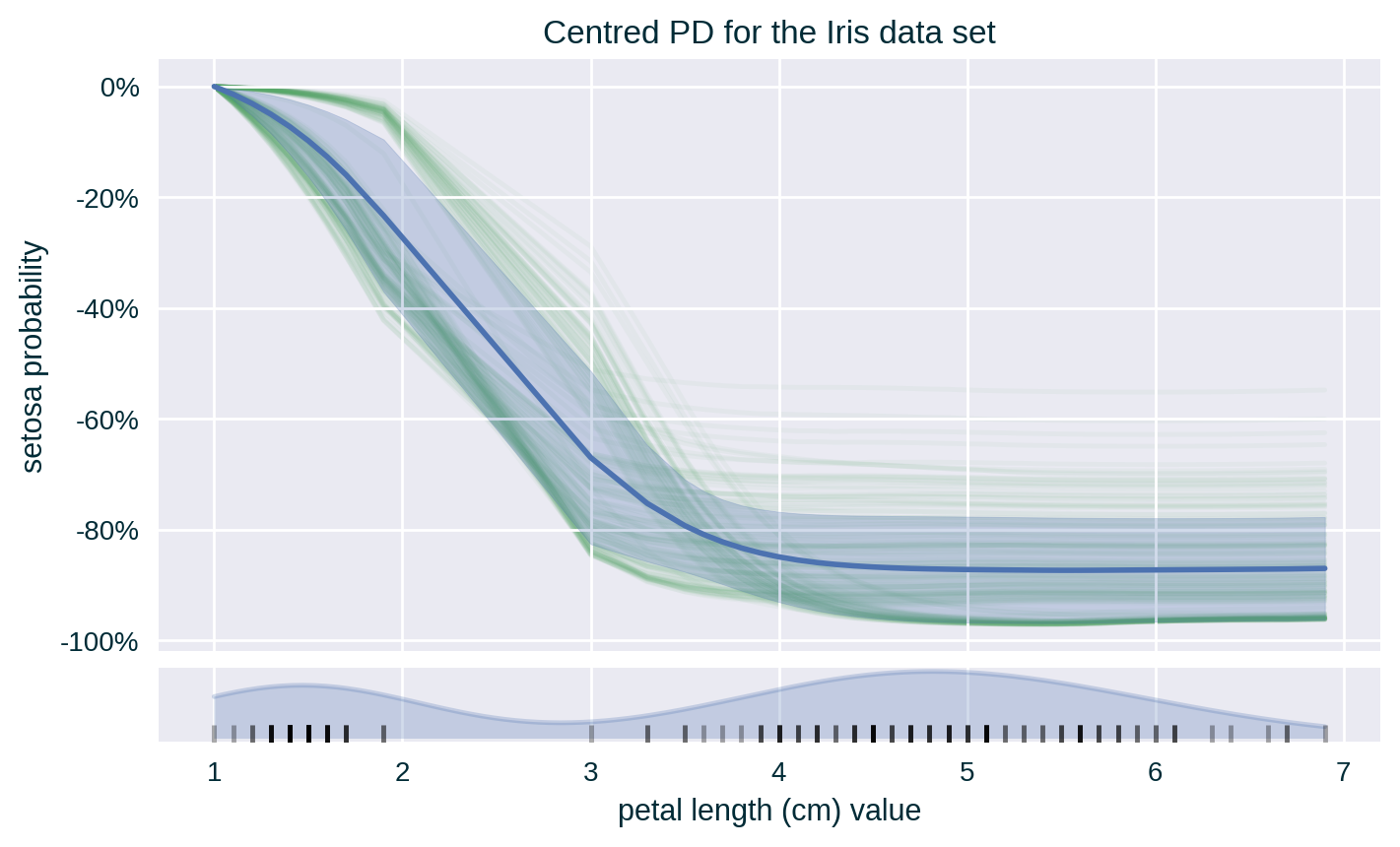
Centres PD curve by anchoring it at a fixed point, usually the lower end of the explained feature range. It is helpful when working with Centred ICE.
\[ \mathbb{E}_{X_{\setminus i}} \left[ f \left( X_{\setminus i} , x_i=V_i \right) \right] - \mathbb{E}_{X_{\setminus i}} \left[ f \left( X_{\setminus i} , x_i=v_i^{\mathit{min}} \right) \right] \]
or
\[ \mathbb{E}_{X_{C}} \left[ \hat{f} \left( x_{S}^{(i)} , X_{C} \right) \right] - \mathbb{E}_{X_{C}} \left[ \hat{f} \left( x^{\star} , X_{C} \right) \right] \]
PD-based Feature Importance
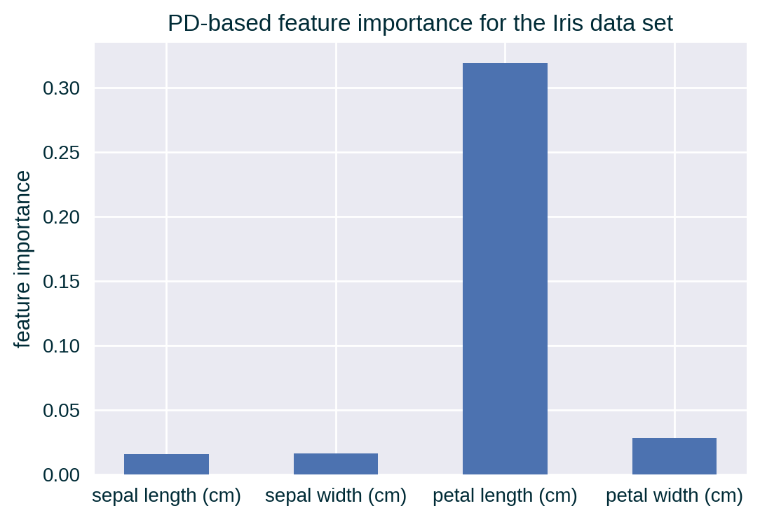
Importance of a feature can be derived from a PD curve by assessing its flatness (Greenwell, Boehmke, and McCarthy 2018). A flat PD line indicates that the model is not overly sensitive to the values of the selected feature, hence it is not important for the model’s decisions.
Caveat
Similar to PD plots, this formulation of feature importance will not capture heterogeneity of individual instances that underlie the PD calculation.
PD-based Feature Importance
For example, for numerical features, it can be defined as the (standard) deviation of PD measurement for each unique value of the explained feature from the average PD.
\[ I_{\mathit{PD}} (i) = \sqrt{ \frac{1}{|V_i| - 1} \sum_{v_i \in V_i} \left( \mathit{PD}_i - \underbrace{ \frac{1}{|V_i|} \sum_{v_i \in V_i} \mathit{PD}_i }_{\text{average PD}} \right)^2 } \]
PD-based Feature Importance
For categorical features, it can be defined as the range statistic divided by four (range rule) of PD values, which provides a rough estimate of the standard deviation.
\[ I_{\mathit{PD}} (i) = \frac{ \max_{V_i} \; \mathit{PD}_i - \min_{V_i} \; \mathit{PD}_i }{ 4 } \]
Formula
For the normal distribution, 95% of data is within ±2 standard deviations. Assuming a relatively small sample size, the range is likely to come from within this 95% interval. Therefore, the range divided by 4 roughly (under)estimates the standard deviation.
PD-based Feature Importance
Based on the ICE notation (Goldstein et al. 2015), where \(K\) is the number of unique values \(x_S^{(k)}\) of the explained feature \(x_S\)
\[ I_{\mathit{PD}} (x_S) = \sqrt{ \frac{1}{K - 1} \sum_{k=1}^K \left( \hat{f}_S(x^{(k)}_S) - \underbrace{ \frac{1}{K} \sum_{k=1}^K \hat{f}_S(x^{(k)}_S) }_{\text{average PD}} \right)^2 } \]
\[ I_{\mathit{PD}} (x_S) = \frac{ \max_{k} \; \hat{f}_S(x^{(k)}_S) - \min_{k} \; \hat{f}_S(x^{(k)}_S) }{ 4 } \]
Examples
PD
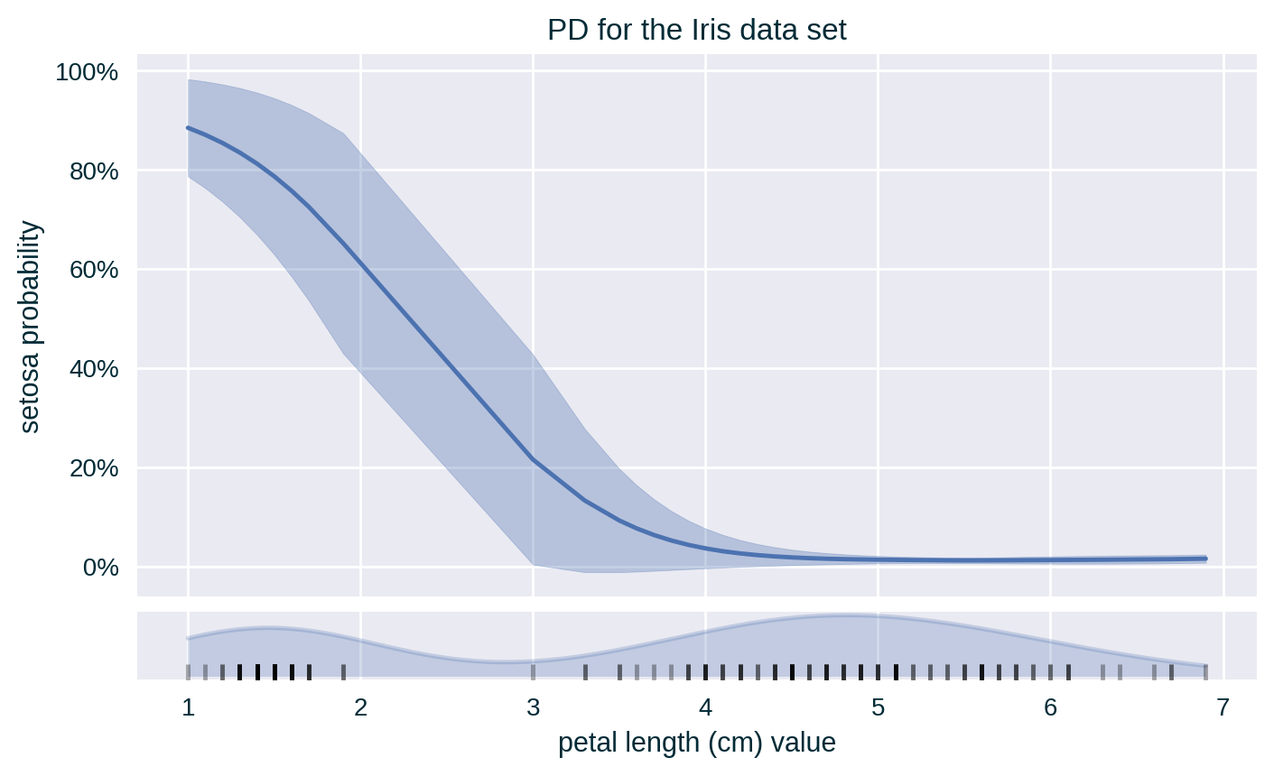
PD with Standard Deviation
PD with ICE
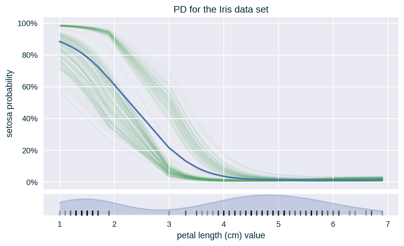
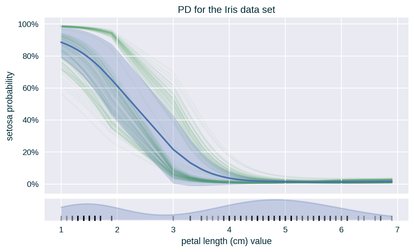
PD with Standard Deviation & ICE
Centred PD (with Standard Deviation & ICE)
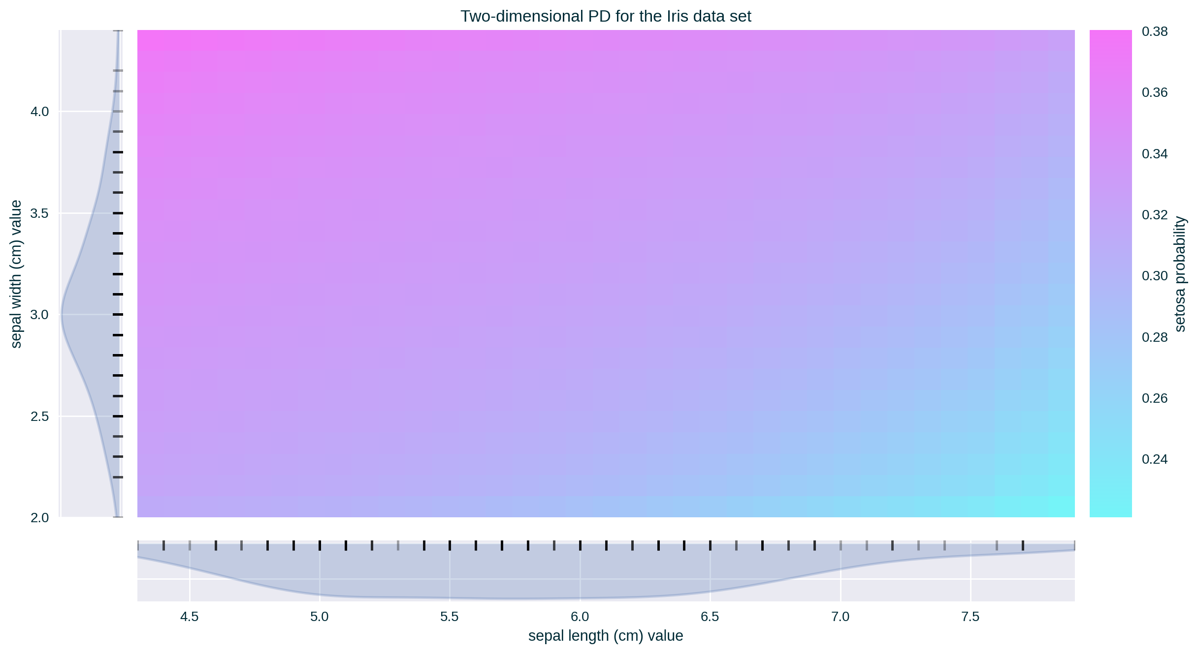
PD for Two (Numerical) Features
PD for Crisp Classifiers
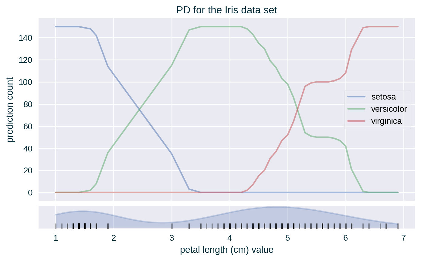
PD for Crisp Classifiers
PD-based Feature Importance
Case Studies & Gotchas!
Out-of-distribution (Impossible) Instances
Feature Correlation
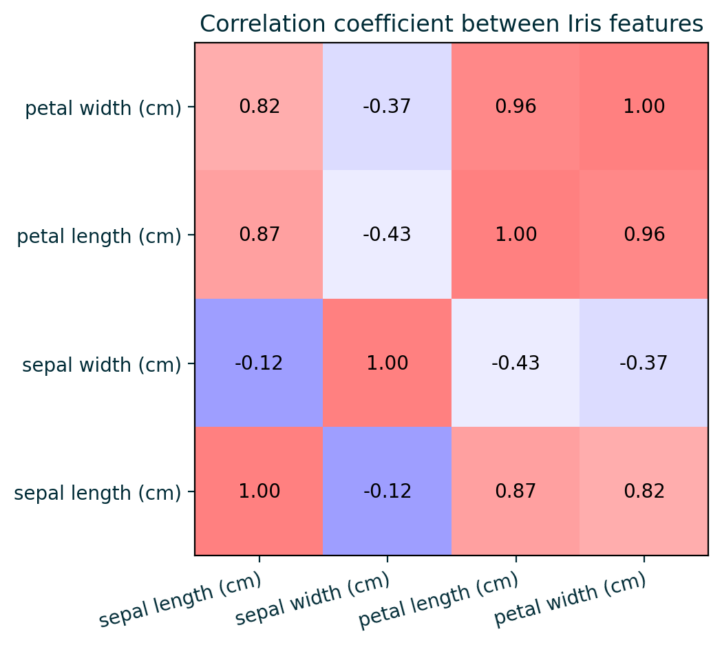
Feature Correlation

Feature Correlation

Feature Correlation

Heterogeneous Influence
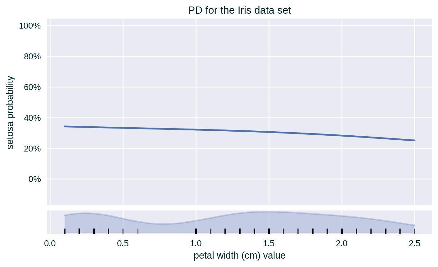
Heterogeneous Influence
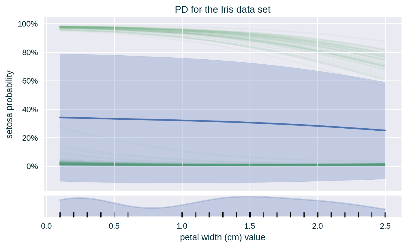
Properties
Pros
- Easy to generate and interpret
- Can be derived from ICEs
- Can be used to compute feature importance
Cons
Assumes feature independence, which is often unreasonable
PD may not reflect the true behaviour of the model since it based upon the behaviour of the model for unrealistic instances
May be unreliable for certain values of the explained feature when its values are not uniformly distributed (abated by a rug plot)
Limited to explaining two feature at a time
Does not capture the diversity (heterogeneity) of the model’s behaviour for the individual instances used for PD calculation (abated by displaying the underlying ICE lines)
Caveats
- PD is derived by averaging ICEs
- Generating PD may be computationally expensive for large sets of data and wide feature intervals with a small “inspection” step
- Computational complexity: \(\mathcal{O} \left( n \times d \right)\), where
- \(n\) is the number of instances in the designated data set and
- \(d\) is the number of steps within the designated feature interval
Further Considerations
Causal Interpretation
Zhao and Hastie (2021) noticed similarity in the formulation of Partial Dependence and Pearl’s back-door criterion (Pearl, Glymour, and Jewell 2016), allowing for a causal interpretation of PD under quite restrictive assumptions:
- the explained predictive model is a good (truthful) approximation of the underlying data generation process;
- detailed domain knowledge is available, allowing us to assess the causal structure of the problem and verify the back-door criterion (see below); and
- the set of features complementary to the explained attribute satisfies the back-door criterion, i.e., none of the complementary features are causal descendant of the explained attribute.
Causal Interpretation
By interveening on the explained feature, we measure the change in the model’s output, allowing us to analyse the causal relationship between the two.
Caveat
In principle, the causal relationship is with respect to the explained model, and not the underlying phenomenon (that generates the data).
Related Techniques
Individual Conditional Expectation (ICE)
Instance-focused (local) “version” of Partial Dependence, which communicates the influence of a specific feature value on the model’s prediction by fixing the value of this feature for a single data point (Goldstein et al. 2015).
Related Techniques
Marginal Effect (Marginal Plots or M-Plots)
It communicates the influence of a specific feature value – or similar values, i.e., an interval around the selected value – on the model’s prediction by only considering relevant instances found in the designated data set. It is calculated as the average prediction of these instances.
Related Techniques
Accumulated Local Effect (ALE)
It communicates the influence of a specific feature value on the model’s prediction by quantifying the average (accumulated) difference between the predictions at the boundaries of a (small) fixed interval around the selected feature value (Apley and Zhu 2020). It is calculated by replacing the value of the explained feature with the interval boundaries for instances found in the designated data set whose value of this feature is within the specified range.
Implementations
| Python | R |
|---|---|
scikit-learn (>=0.24.0) |
iml |
| PyCEbox | ICEbox |
| PDPbox | pdp |
| InterpretML | DALEX |
| Skater | |
| alibi |
Further Reading
- PD paper (Friedman 2001)
- Interpretable Machine Learning book
- Explanatory Model Analysis book
- Kaggle course
- scikit-learn example
- FAT Forensics example and tutorial
- InterpretML example